
Expectation and Variance of Uniform distribution
Contents:
1. Review
1.1. Uniform distribution
a. Discrete Uniform distribution
$ \textbf{Notation: }\mathcal{U}\{a, b\} \text { or unif}\{a, b\} $
Probability Mass Function (PMF):
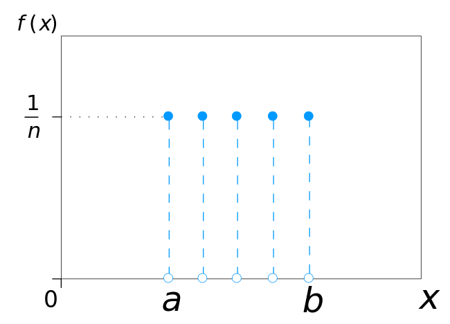
\(\text { PMF of the discreet uniform distribution: } f(x)=\left\{\begin{array}{ll}{\frac{1}{b-a+1}} & {\text { for } x \in[a, b] \text{, } x \in \mathcal{Z}} \\ {0} & {\text { otherwise }}\end{array}\right.\)
Examples:
- $ \text{Toss a cube, the probability to get each of 6 sides is equal to each other and equal to }\frac{1}{6}$.
- A class has 4 groups with the same number of students. Random varibale $ X $: choose randomly 1 student in the class. The probability such that that student in each group is equal to each other.
b. Continuous Uniform distribution
$ \textbf{ Notation } \quad \mathcal{U}(a, b) \text { or unif}(a, b) $
Probability Density Function (PDF):
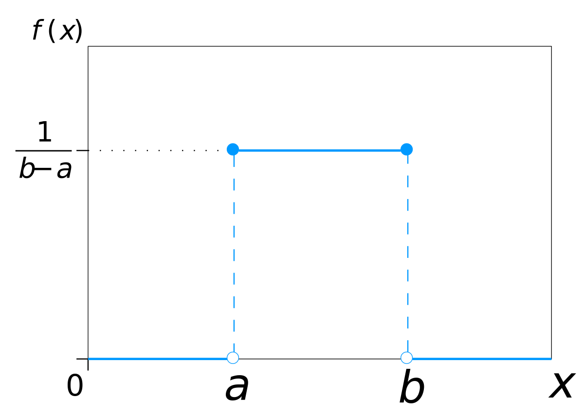
Continuous Uniform distribution is also called rectangular distribution because of its shape.
1.2. Expectation
Expectation or Expected value is the weighted average value of a random variable.
a. Discrete random variable
\[E[X]=\sum_{i} x_{i} P(x)\]$ E[X] \text { is the expectation value of the continuous random variable X} $
$ x \text { is the value of the continuous random variable } X $
$ P(x) \text { is the probability mass function of (PMF)} X $
b. Continuous random variable
\[E(X)=\int_{-\infty}^{\infty} x P(x) d x\]$ E(X) \text { is the expectation value of the continuous random variable } X $
$ x \text { is the value of the continuous random variable } X $
$ P(x) \text { is the probability density function (PDF) } $
Properties: $ \text{When } a \text{ is a constant and }X, Y \text{ are random variables:} $
- Linearity
$ E[a X]=a E[X] $
$ E[X+Y]=E[X]+E[Y] $
- Constant
$ E[a]=a $
1.3. Variance
$ \begin{array}{l}{\text { The variance of random variable } X \text { is the expected value of squares of difference of } X \text { and }} \ {\text { the expected value } \mu .}\end{array} $
\[\sigma^{2}=\operatorname{Var}(X)=E\left[(X-\mu)^{2}\right]\]This is equivalent to:
\[\sigma^{2}=\operatorname{Var}(X)=E\left[X^{2}\right]-\mu^{2}\]Properties: where $C$, $a$, $b$ are constants
- $\operatorname{Var}(X+C) = \operatorname{Var}(X)$
- $\operatorname{Var}(CX)=C^{2}.\operatorname{Var}(X)$
- $\operatorname{Var}(aX + b)=a^{2}.\operatorname{Var}(X)$
- $\operatorname{Var}(X_{1}+X_{2}+…+X_{n})=\operatorname{Var}(X_{1})+\operatorname{Var}(X_{2})+…+\operatorname{Var}(X_{n})$ if $X_{1}, X_{2},…, X_{n}$ are independent random variables.
2. Expectation of Uniform distribution
Continuous distribution: \(E(X)=\int_{-\infty}^{\infty} x P(x)dx=\int_{a}^{b} x \frac{1}{b-a} dx\) \(\iff E(X) = \frac{1}{2(b-a)}*x^{2}\vert_{a}^{b} = \frac{a+b}{2}\)
Discrete Uniform distribution:
\[E[X] = \sum_{a}^{b} xP(x) = \frac{1}{b-a+1}[a+(a+1)+(a+2)+...+b]\] \[E[X] = \frac{1}{b-a+1}\frac{(a+b)(b-a+1)}{2} = \frac{a+b}{2}\]$ \text{Therefore, in discrete uniform distribution: } E[X] = \frac{a+b}{2} $
3. Variance of Uniform distribution
Continuous Uniform Distribution:
\[\operatorname{Var}(X)=E\left[X^{2}\right]-\mu^{2} = E[X^{2}] - \frac{(a+b)^{2}}{4}\]Let’s calculate $ E[X^{2}] $
\[E[X^{2}] = \int_{a}^{b}\frac{x^{2}}{b-a} dx = \frac{b^{3}-a^{3}}{3(b-a)}=\frac{a^{2}+ab+b^{2}}{3}\]Hence,
\[\operatorname{Var}(X)=\frac{a^{2}+ab+b^{2}}{3} - \frac{(a+b)^{2}}{4} = \frac{(b-a)^{2}}{12}\]Discrete Uniform distribution: \(\operatorname{Var}(X)=E\left[X^{2}\right]-\mu^{2} = E[X^{2}] - \frac{(a+b)^{2}}{4}\)
$ \text{To calculate } \operatorname{Var}(X) \text{, we find } E[X^{2}] $
\[E[X^{2}] = \frac{1}{b-a+1}*[a^{2}+(a+1)^{2} + ... + b^{2}] (1)\]$ \text{Let } S(n)=1^{2}+2^{2}+3^{2}+…+n^{2} \text{, so }(1) \iff E[x^{2}]=\frac{S(b)-S(a-1)}{b-a+1} $
On the other hand: $ n^{2} < S(n)=1^{2}+2^{2}+3^{2}+…+n^{2} < n^{3} $
$ \text{Hence, if there is a rule for } S(n) \text{, it must be in this form: } S(n)=xn^{3} + yn^{2} + zn + t \text{ (2)} $
\[S(n+1) = S(n) + (n+1)^{2} \iff x(n+1)^{3} + y(n+1)^{2} + z(n+1) + t = xn^{3} + yn^{2} + zn + t + (n+1)^{2}\] \[\iff xn^{3} + (3x+y)n^{2} + (3x+2y+z)n + (x+y+z) = xn^{3} + (y+1)n^{2} + (z+2)n +1\] \[\left\{\begin{array}{l}{3x+y=y+1} \\ {3x+2y+z=z+2} \\ {x+y+z=1}\end{array}\right. \iff \left\{\begin{array}{l}{x=\frac{1}{3}} \\ {y=\frac{1}{2}} \\ {z=\frac{1}{6}}\end{array}\right.\]$ \text{Substitute these values in (2): } S(n) = \frac{1}{3}n^{3}+\frac{1}{2}n^{2}+\frac{1}{6}n+t \text{. Additionally, }S(1) = 1 \text{ so } t=0. $
$ \text{Finally, } S(n) = \frac{1}{3}n^{3}+\frac{1}{2}n^{2}+\frac{1}{6}n $
$ \text{Now we can calculate } E[X^{2}] $
$ E[X^{2}]=\frac{1}{b-a+1}\{\frac{1}{3}[b^{3}-(a-1)^{3}]+\frac{1}{2}[b^{2}-(a-1)^{2}]+\frac{1}{6}[b-(a-1)]\} $
\[=\frac{1}{3}[b^{2}+b(a-1)+(a-1)^{2}] + +\frac{1}{2}(b+a-1)+\frac{1}{6}\] \[=\frac{2b^{2}+2ab-2b+2a^{2}-4a+2+3b+3a-3+1}{6} = \frac{2a^{2}+2b^{2}+2ab-a+b}{6}\]$ \text{And finally, } \operatorname{Var}(X) $
\[\operatorname{Var}(X)= E[X^{2}] - \frac{(a+b)^{2}}{4} = \frac{2a^{2}+2b^{2}+2ab-a+b}{6} - \frac{(a+b)^{2}}{4}\] \[\operatorname{Var}(X)= \frac{4a^{2}+4b^{2}+4ab-2a+2b-3a^{2}-3b^{2}-6ab}{12} = \frac{(b-a)^{2}+2(b-a)}{12}\] \[\operatorname{Var}(X)= \frac{(b-a)(b-a+2)}{12}\]